How do I decide Unit; Criterion C: Creating Solution

How do I decide Unit; Criterion C: Creating Solution

Follow the checklist below as you work on the creation of your solution

• The Plan:
• I have constructed a logical plan (a step-by-step procedure) for the creation of the solution.  (sufficient for peers to be able to follow)
• I have stated the resources that will be needed.
• I have completed a timeline / Gantt chart
• The Creation Process:
  • I have demonstrated excellent technical skills when making the solution.
  • I have fully justified changes made to the chosen design and plan when making the solution.
• Process Journal: 

                        I have maintained a process journal through the entire creation process.

• I have explained the tools and techniques used in the process of creation.
• I have included evidence in the creation phase that I have followed my time plan.
• I have reflected any changes I made to my plan during the creation phase.
• I have included screen shots and other photographic evidences of the key phases of creation.
• I have kept notes in my process journal about how well I worked, problems encountered, and use of time - to be used in the evaluation.
• The Final Project: I have presented the solution as a whole, either in electronic form, or through photographs of the solution from different angles, showing details.
• Evaluate: I have evaluated and reflected on my performance in the this stage.
• Challenges and successes
• Areas of concerns
• The strengths and weaknesses.
• Observations on how this stage could have been improved.
• General reflections 

Requirements for each strand 

(i) Construct a logical plan that describes the efficient use of time and 

resources, sufficient for peers to be able to follow to create the solution. 

pages 1- 2

By the end of year 4 you should be able to:

• construct a series of logical steps to create the solution, using charts, diagrams and text that include aspects of quality control and quality assurance
• construct a plan to create the solution that makes effective use of resources and time
• construct a clear and concise plan that peers will be able to follow to create the solution

(ii) Demonstrate excellent technical skill when making the solution

At the end of year 4 you should be able to:

• develop manipulative skills to effectively use a wide range of tools, techniques and equipment
• use a wide range of tools and equipment proficiently to create high-quality solutions
• ensure a safe working environment for themselves and others

(iii) Follow the plan to create the solution, which functions as intended

By the end of year 4 you should be able to:

• independently follow the plan to produce the solution, which functions as intended
• manage time effectively to produce the solution to the deadline stated in the plan

 ( strand 2 and 3. At-least 6 Pages)

(iv) Fully justify changes made to the chosen design and plan when making the solution

By the end of year 4 you should be able to: Pages 2 or 3 pages

• justify, through the use of drawings/diagrams, any changes made to the design while making the solution and how they affected the plan

Criterion B: Developing Ideas

Criterion B: Developing Ideas

At the end of year 5, students should be able to:

i. develop design specifications, which clearly states the success criteria for the design of a solution

ii. develop a range of feasible design ideas, which can be correctly interpreted by others

iii. present the chosen design and justify its selection

iv. develop accurate and detailed planning drawings/diagrams and outline the requirements for the creation of the chosen solution.


Strand i)

i)   develop design specifications, which clearly states the success criteria for the design of a solution

-      The design specs should be measurable with a clear way on how the specs will be tested.

-      The specification should be directly connected to your design brief. 

Example: Game Product

Specification	Test
Game will be less than 1 MB in size	Install it in a computer  the size in properties
Played by two players (Multiplayer game)	Allow two players to play simultaneously
The game 3 levels that will advance in complexity.	Play the game at each level time the duration it takes to complete a level and record the complexities.

Maximum of 2 pages

Strand ii) 

ii) develop a range of feasible design ideas, which can be correctly interpreted by others

- Develop a range of good quality designs and measure each of them against the design specs.

- Your description for each design should be detailed and clear and use captions on images or diagrams which are not clear.

- Annotate  the designs with sufficient detail to explain how they meet the requirements of the design specification and to explain design thinking

Sketches
https://sketchboard.io/

https://sketch.io/sketchpad/

Examples of Designs

Maximum of  7 pages

Strand iii)

iii.           present the chosen design and justify its selection

         -      State the chosen design.

         -      Provide detailed justification why the design was chosen.

         -      Suggest possible improvements to the chosen design. 

         -      If possible show the chosen design with the improvements included as a final design.

Maximum of  2 pages 

Strand iv)
iv.           develop accurate and detailed planning drawings/diagrams and outline the requirements for the creation of the chosen solution.
          
          The above can be achieved using either of the following tools
           a) Table of requirements.
b)  Flowchart
c)  Site Map

 This should not be confused with the designs developed and justified. This is the process detailing the requirement for the creation of the chosen solution.  

Site Map

Flowchart Sketching software
https://www.digikey.com/schemeit/project/

Site Map Builders
https://www.gloomaps.com/

Maximum of 4 pages

Resouce blog

http://robc84.wixsite.com/bisdesign/copy-of-crit-b-4

How to Sort Data in Excel Spreadsheets (The Right Way)

So, you get handed an Excel spreadsheet with thousands of rows inside of it, and you realize the data is all out of order. You might need to sort it based on the names inside of a column, or by sorting data from large to small.

On the surface, sorting data is a simple task in Excel, and the app certainly makes simple sorting easy. However, there's much more power in how you can sort and reorder the data in your worksheets. Here are three Excel data sorting techniques you'll learn in this tutorial:

1. Sort data simply with just a couple of clicks.

A Simple Sort in Excel

Sorting can be a very simple, two-click process to reorganize the data in your spreadsheet. Let's learn how.

In an Excel workbook, start off by clicking in a cell of the column you want to sort. Now, make sure that you're on the Home tab of Excel's ribbon, and find the Sort and Filter button on the far right side of it.

The Sort & Filter button lives on the far right side of the Home tab on the ribbon.

Notice that in the sort options, you can sort text "A to Z", or "Z to A." These simple options will alphabetically sort the Excel data either direction, depending on the option you choose.

When you are sorting data in Excel, the entire row is being sorted. Essentially, the column you select will be the "key" that Excel uses that to decide how to sort the data, but each row is a record that should stay grouped together.

Depending on the data you've selected, you can sort alphabetically or numerically. If your column has numerical values, you can sort from smallest to largest amounts, while text data will sort based on alphabetical order.

In the example above, the sort options have changed because I've selected a column with numbers.

It really is this easy to perform a basic sort. Simply click inside of a column of data, choose a sort option, and Excel will reorder the data inside a spreadsheet.

Advanced Excel Data Sorting

So far, a simple sort has allowed us to sort for a single type of data. What if we want to consider two types of data in our sorting?

What if we wanted to...

• Sort alphabetically by the state, and then by the county in a spreadsheet.
• Sort alphabetically by the name of a client, and then by each type of project we did for them.
• Sort our clients in a list alphabetically, and then by amount for each individual project, from largest to smallest.

The answer to all of these is an advanced sort, where you can set multiple levels of sorting data. Let's walk through that last example using the sample data.

To get started, click somewhere inside of your data and find the Sort & Filter option, and then choose Custom Sort.

Access advanced sorting options by choosing Sort & Filter > Custom Sort.

On this window, we can add multiple levels of sorting. Start off by clicking on the dropdown option next to Sort by and choose a column that you want to sort by.

In my case, I'll choose Client from the dropdown menu, and leave the the Sort On set to Values, and Order set to A to Z. In plain English, this will sort the Excel spreadsheet based on alphabetical order.

Now, let's click on Add Level. This will create a new row in the sort options and allows us to add a second level of organization.

I can now choose Amount billed from the second dropdown. The combination of these two rules will start by sorting based on the client name, and then by the amount billed on each project.

You could continue to add as many levels as you want to this advanced sorting window. The sequence of the rows matters; you can move a row up to sort first by the amount billed, for example, and then by client.

Once we press OK, Excel will sort the spreadsheet based upon the rules we've built in this window.

Using functions and nested functions in Excel formulas

Functions are predefined formulas that perform calculations by using specific values, called arguments, in a particular order, or structure. Functions can be used to perform simple or complex calculations. You can find all of Excel's functions on the Formulas tab on the Ribbon:

IF FUNCTION IN EXCEL.

The IF function is one of the most popular and useful functions in Excel. You use an IF statement to ask Excel to test a condition and to return one value if the condition is met, and another value if the condition is not met.

The IF function is one of Excel's logical functions that evaluates a certain condition and returns the value you specify if the condition is TRUE, and another value if the condition is FALSE.

The syntax for Excel IF is as follows:

IF(logical_test, [value_if_true], [value_if_false])

As you see, the IF function has 3 arguments, but only the first one is obligatory, the other two are optional.

• logical_test - a value or logical expression that can be either TRUE or FALSE. Required.In this argument, you can specify a text value, date, number, or any comparison operator.
  For example, your logical test can be expressed as or B1="sold", B1<12/1/2014, B1=10 or B1>10.
• value_if_true - the value to return when the logical test evaluates to TRUE, i.e. if the condition is met. Optional.
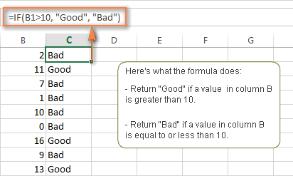
  For example, the following formula will return the text "Good" if a value in cell B1 is greater than 10: =IF(B1>10, "Good")
• value_if_false - the value to be returned if the logical test evaluates to FALSE, i.e. if the condition is not met. 

Using the IF function in Excel - formula examples

Now that you are familiar with the Excel IF function's syntax, let's look at some formula examples and learn how to use IF as a worksheet function in Excel.

Excel IF statement for numbers: greater than, less than, equal to

The use of the IF function with numeric values is based on using different comparison operators to express your conditions. You will find the full list of logical operators illustrated with formula examples in the table below.

Condition	Operator	Formula Example	Description
Greater than	>	=IF(A2>5, "OK",)	If the number in cell A2 is greater than 5, the formula returns "OK"; otherwise 0 is returned.
Less than	<	=IF(A2<5, "OK", "")	If the number in cell A2 is less than 5, the formula returns "OK"; an empty string otherwise.
Equal to	=	=IF(A2=5, "OK", "Wrong number")	If the number in cell A2 is equal to 5, the formula returns "OK"; otherwise the function displays "Wrong number".
Not equal to	<>	=IF(A2<>5, "Wrong number", "OK")	If the number in cell A2 is not equal to 5, the formula returns "Wrong number "; otherwise - "OK".
Greater than or equal to	>=	=IF(A2>=5, "OK", "Poor")	If the number in cell A2 is greater than or equal to 5, the formula returns "OK"; otherwise - "Poor".
Less than or equal to	<=	=IF(A2<=5, "OK", "")	If the number in cell A2 is less than or equal to 5, the formula returns "OK"; an empty string otherwise.

Excel IF function examples for text values

Generally, you write an Excel if statement with text using either "equal to" or "not equal to" operator, as demonstrated in a couple of IF examples that follow.

Example 1. Case-insensitive IF formula for text values

Like the overwhelming majority of Excel functions, IF is case-insensitive by default. What it means for you is that logical tests for text values do not recognize case in usual IF formulas.

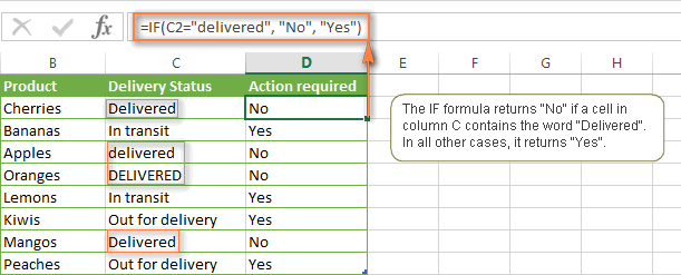
For example, the following IF formula returns either "Yes" or "No" based on the "Delivery Status" (column C):

=IF(C2="delivered", "No", "Yes")

Translated into the plain English, the formula tells Excel to return "No" if a cell in column C contains the word "Delivered", otherwise return "Yes". At that, it does not really matter how you type the word "Delivered" in the logical_test argument - "delivered", "Delivered", or "DELIVERED". Nor does it matter whether the word "Delivered" is in lowercase or uppercase in the source table, as illustrated in the screenshot below.

READ MORE ON IF FUNCTION CLICK HERE

CELL RANGE, CELL REFERENCING (RELATIVE AND ABSOLUTE CELL REFERENCING)

CELL RANGE, CELL REFERENCING (RELATIVE AND ABSOLUTE CELL REFERENCING)

Cell Range

While references often refer to individual cells – such as A1, they can also refer to a group or RANGE of cells.

Ranges are identified by the cell references of the cells in the upper left and lower right corners of the range.

The two cell references used for a range are separated by a colon ( : ) which tells Excel or Google Sheets to include all the cells between these start and end points

e.g =sum( D3:D10)

Relative, Absolute, and Mixed Cell References

The three types of references that can be used in Excel and Google Sheets are easily identified by the presence or absence of dollar signs ($) within the cell reference:

• Relative cell references Used to copy formulas into other cells and contain no dollar signs, as shown in the formula in row 2, = A2+A4.
• This means the formulas will follow similar operation while being used. Such operations can cause errors in the calculations.
• Absolute cell references  used to copy formulas into other cells without causing errors and changes. They use dollar signs to each letter or number in a reference, as shown in the formula in row 4, =$A$2+$A$4.
• Mixed cell references have dollar signs attached to either the letter or the number in a reference but not both, as shown in the formula in row 5, =$A2+A$4.
• SEE THIS LINK

Copying Formulas and Different Cell References

Another advantage of using cell references in formulas is that they make it easier to copy formulas from one location to another in a worksheet or workbook.